What Thousands of Steel-Plant Drone Frames Reveal About the Camera and AI You Actually Need

The short version

A close-up in an inspection report is usually a crop of the wide photo. Detail the camera did not record cannot be added back.
Work backwards from the defect. At 17 m, a 20 MP camera with 1.4 µm pixels and a 6 mm lens records about 4 mm per pixel.
At that size, lifted and missing sheets are easy to see. A 10 mm hole is at the edge of what can be spotted, and cracks cannot be measured.
Many serious defects sit on walls, corners and gable ends, so fly side-on views as well as the roof.
Light ruins more frames than resolution does: backlight, deep shade and dust.
Motion, lens sharpness and the data link all take pixels away or add cost, and each can be calculated before the first flight.
To know how often a camera finds a defect, plant known defects on a test wall and count.

Open almost any drone inspection report and you will find the same page: a wide photo with a red box, a zoomed close-up beside it, a severity rating and a recommendation.

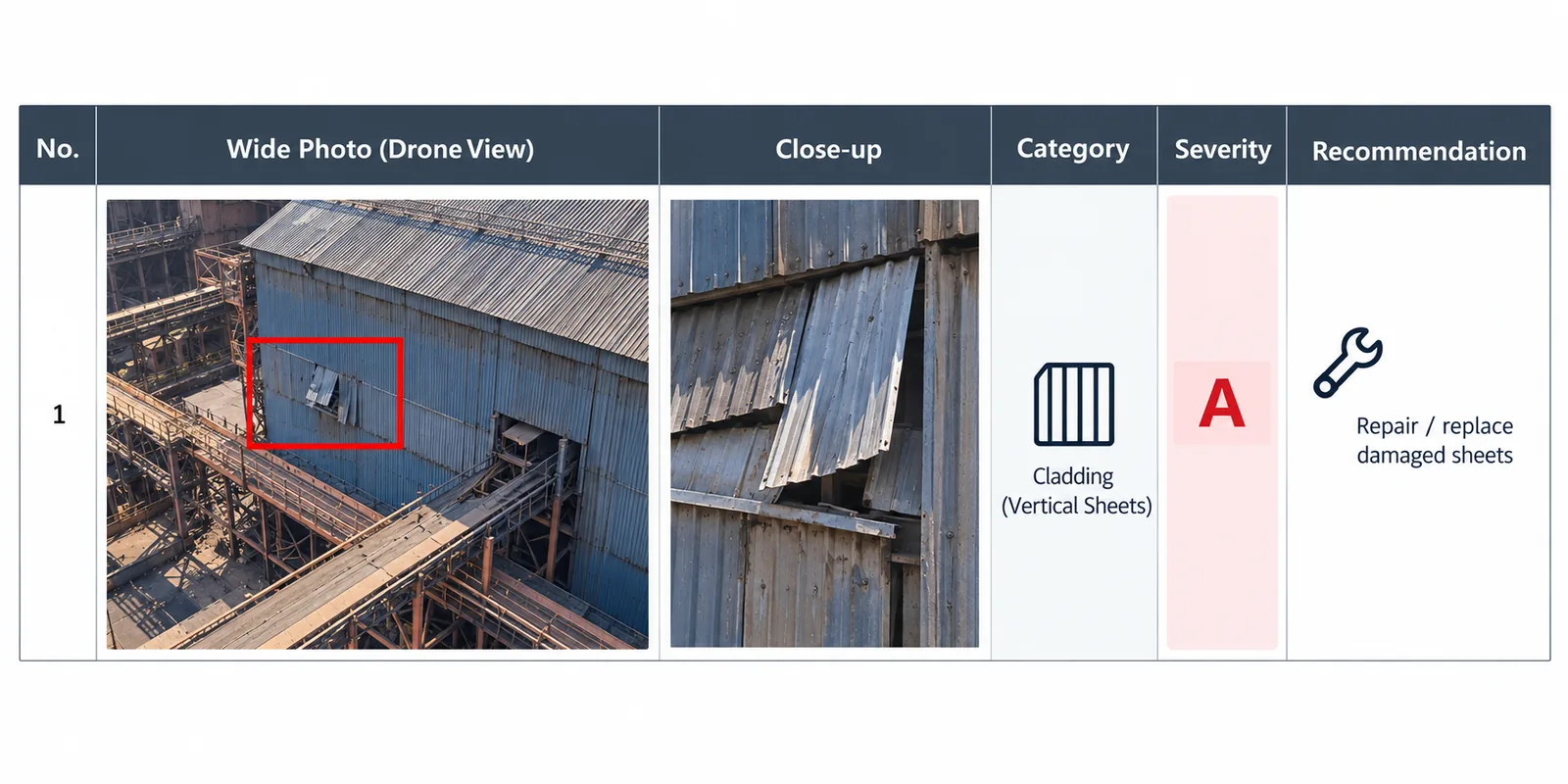
A typical inspection report row: wide drone view with a red box, a zoomed close-up of the same frame, the category, a severity letter and a recommendation — A typical report row. The close-up on the right is usually a crop of the wide frame, not a second photo.

That close-up is rarely a second photo taken from nearer. It is the same photo, enlarged on screen, so whatever the camera did not record the first time is gone for good.

The pixel count is the most zoom an inspector will ever have.

So the useful question is what the camera has to record for a finding to hold up.

Start from the defect

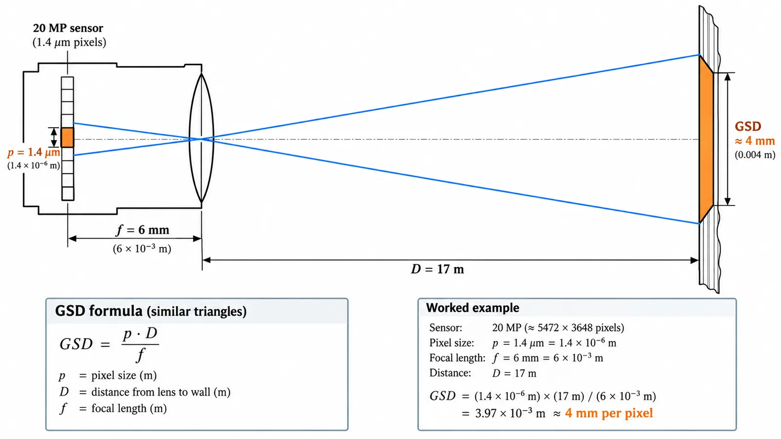
The first number to know is how many millimetres of the structure one pixel covers. Surveyors call this the ground sample distance, or GSD.

Two details matter. The distance is the straight line from the lens to the surface, not the drone’s height: a drone 110 m up beside a chimney and 20 m from the steel is working at 20 m. And the lens counts as much as the sensor, because the same camera with a wider lens sees more area in less detail.

GSD (mm/px) = distance × pixel size ÷ focal length

Our worked example is a 20 MP sensor with 1.4 µm pixels and a 6 mm lens, 17 m from a wall. It gives 3.97 mm per pixel, which we round to 4 mm and use throughout. The sensor is the onsemi AR2020, the one e-con Systems fits in its e-CAM200 module. The pixel budget card further down runs the same sum for any camera, lens and distance.

20 MP AR2020
e-CAM200_CUMI2020C_MOD
5120 × 3840 · 1.4 µm · rolling shutter · 30 fps at 20 MP
4.0 mm/pxat 17 m with a 6 mm lens, 20.3 m across
Product page

Similar-triangles diagram: a 20 MP sensor with 1.4 µm pixels and a 6 mm lens at 17 m from a wall; each pixel covers about 4 mm — Similar triangles: one 1.4 µm pixel behind a 6 mm lens covers 3.97 mm of wall at 17 m.

The emergencies are on the walls

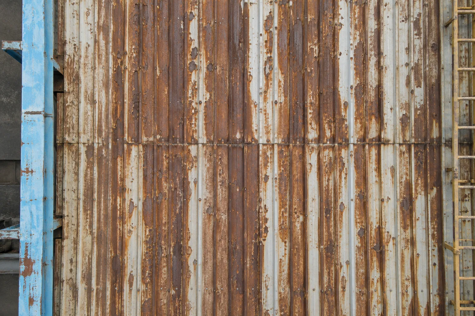
A neat top-down grid is the natural flight plan, the way a mapping survey works. But many of the defects that matter on industrial buildings are on the sides. Wind suction is strongest at roof edges and corners, which is where cladding and flashing work loose, and you cannot see a wall from straight above.

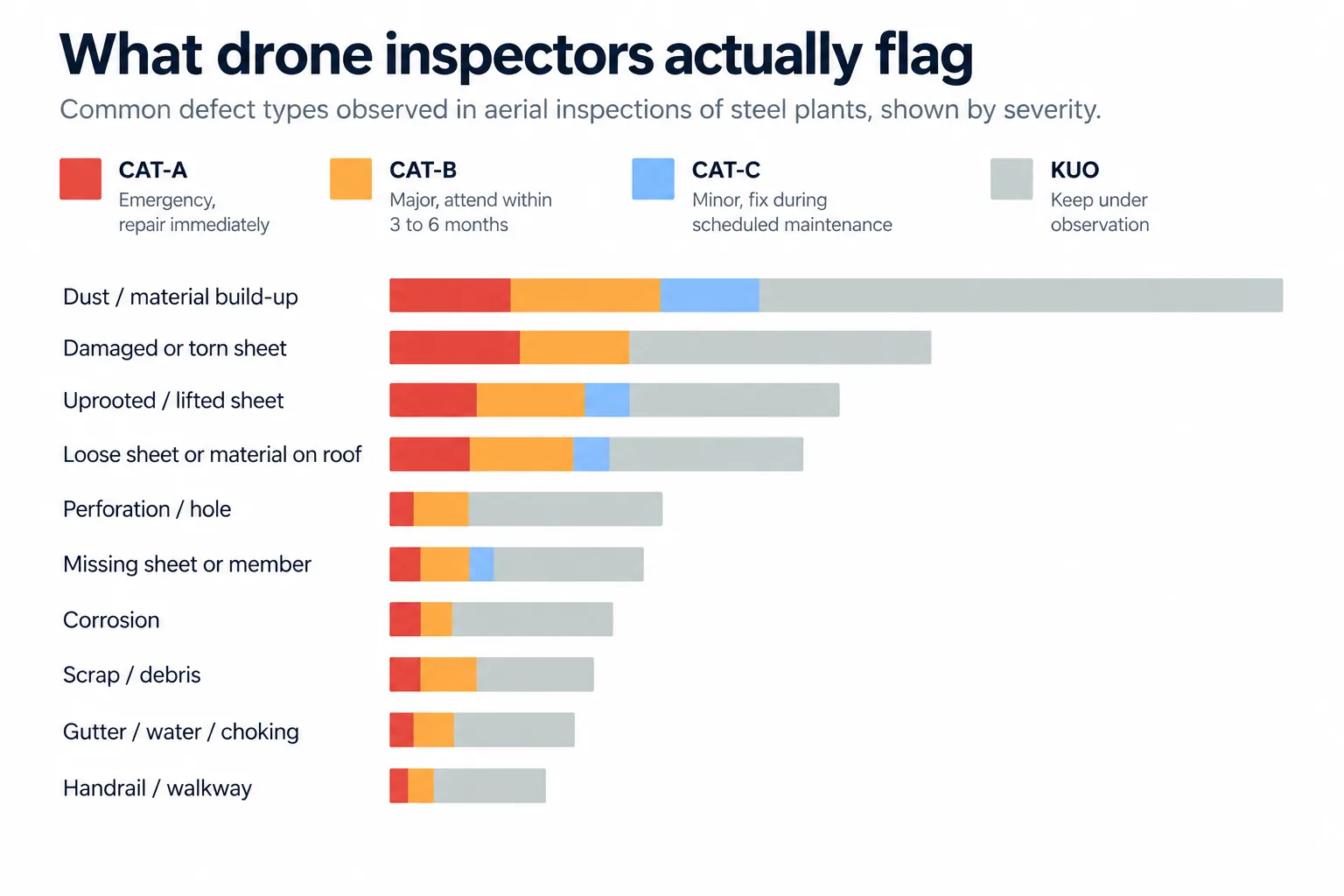
Lifted and uprooted sheets dominate the emergencies

Uprooted or lifted sheets45%

Damaged sheets25%

Loose material on roofs20%

Perforations9%

Missing sheets5%

Corrosion3%

Share of CAT-A (emergency) findings that involve each defect type in the analysed missions. The shares add to more than 100 % because a finding can involve more than one type.

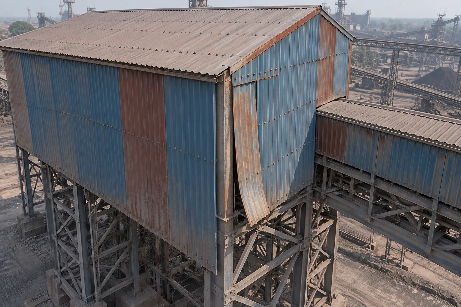
Vertical side cladding was named in several CAT-A entries, ahead of roof sheets, flashing and louvres, and the locations cluster at gable ends, corners and around ducts. Dust and material build-up was the most common finding overall at 36 %, but only 9 % of those were CAT-A.

Stacked bar chart of drone inspection findings by type and severity, from dust and material build-up at the top to handrail and walkway at the bottom — What drone inspectors flag, split by severity from CAT-A (act now) to keep under observation.

The flight logs agree. The median camera tilt was −30°, only 13 % of frames were close to straight down, and on stack missions 11 % looked upward.

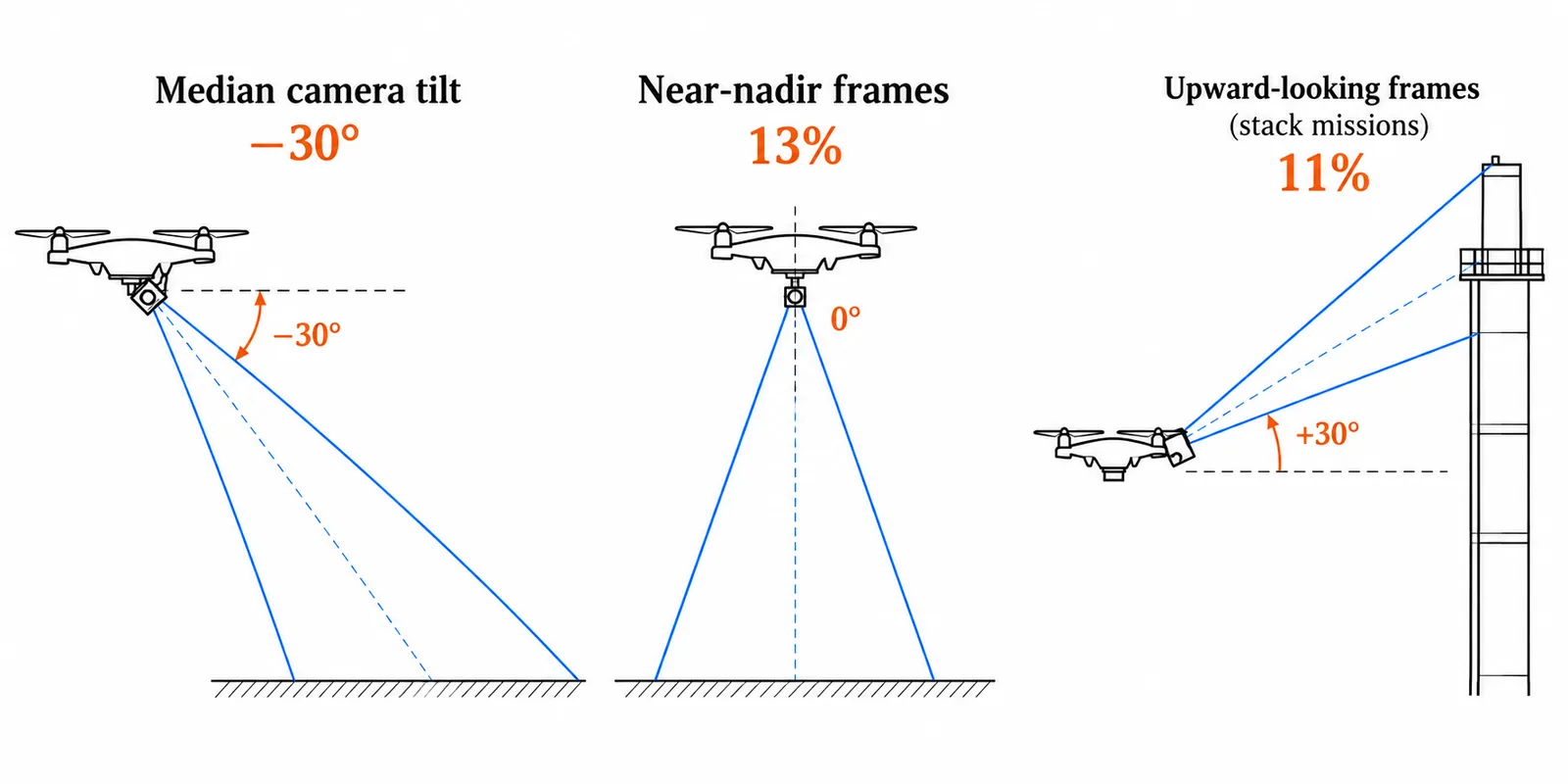
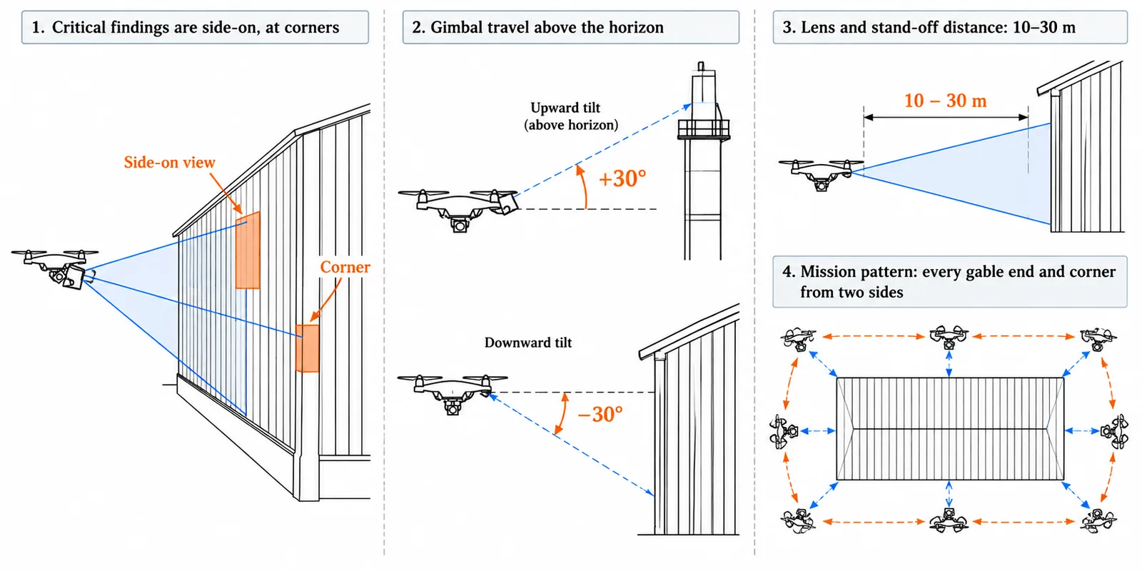
Three drone sketches: median camera tilt −30°, 13% near-nadir frames, 11% upward-looking frames on stack missions — Where the camera actually pointed, from flight metadata.

The findings that matter are side-on, at corners and in mixed light, so the camera, gimbal and flight plan should be built for those views.

In practice that means a gimbal that tilts above the horizon, lenses chosen for 10 to 30 m stand-off instead of 100 m altitude, and a flight pattern that shoots every gable end and corner from two sides.

Mission design: side-on views at corners, gimbal travel above the horizon, 10 to 30 m stand-off, and an orbit that shoots every gable end and corner from two sides — Designing the mission around side-on findings.

Weathered blue and rust-coloured cladding on a raised industrial building, with a sheet lifting at the gable end — Gable ends and corners are where cladding works loose.

What 4 mm per pixel can and cannot show

Imaging science has a long-standing rule of thumb, the Johnson criteria. To have even odds of completing a task, you need about 2 pixels across the narrowest side of the target to spot it, 8 to classify it and 13 to identify it. The rule was fitted to people looking at vehicles, so treat it as a guide for planning. For a more cautious plan, move to the 90 % level, which needs about 3.5, 14 and 23 pixels.

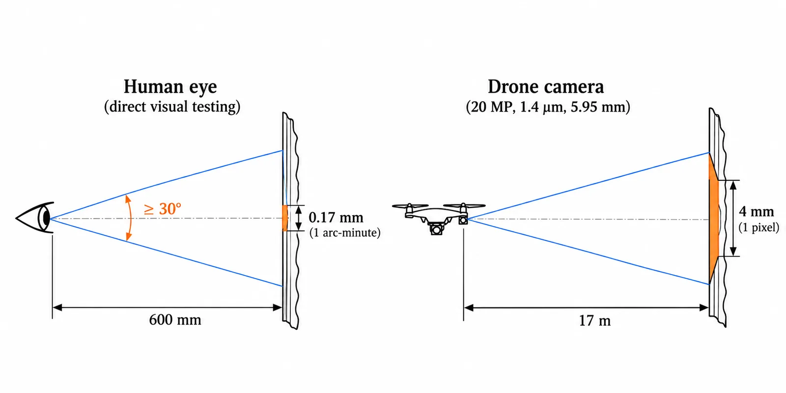
Hands-on visual inspection is usually done within about 600 mm, where normal eyesight resolves about 0.17 mm. Our drone camera records 4 mm per pixel, about 23 times coarser. To match the eye at 600 mm you would have to fly within 0.73 m of the surface, or 1.5 m with a 12 mm lens. Nobody does that along a conveyor gallery.

Human eye at 600 mm resolves 0.17 mm; drone camera at 17 m records 4 mm per pixel — The eye at 600 mm against the drone camera at 17 m.

Sheet-level defects, which drive most CAT-A findings, are well inside the limit. A missing sheet covers hundreds of pixels.

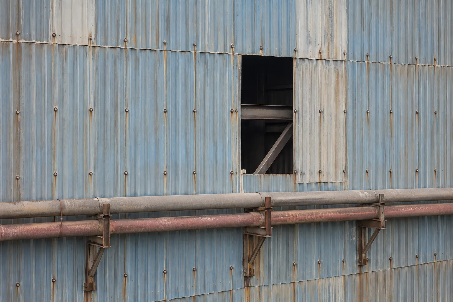
A missing cladding sheet leaves a dark rectangular opening in a corrugated wall — A missing sheet spans hundreds of pixels at 4 mm per pixel.

Holes are a different story. A 10 mm perforation covers about 2.5 pixels, which is at the edge of what can be spotted. A 60 mm hole covers about 15, enough to classify. A 0.3 mm crack is a fraction of one pixel wide, so at any practical stand-off it cannot be measured or classified. A long, high-contrast line can sometimes still be spotted, and then the drone flags the area and a technician measures it.

The card below shows how many pixels a detail gets. It starts with the e-CAM200 sensor at 17 m with a 6 mm lens, looking at a 10 mm hole.

Pixel budget

Camera

Camera sensor

Focal length mm

The real value, not the 35 mm equivalent.

Distance m

Straight line from the lens to the subject.

Detail

Smallest detail mm

Its narrowest side.

Task

Smallest detail you can classify at 17.0 m

56 mm

Ground sample distance3.97 mm/px
Frame width20.3 m
Pixels needed to classify14.0 px90 % confidence
Your 10.0 mm detail2.5 pxlongest distance 3.1 m

Common details at this pixel size

Detail	Size	Pixels across	Longest distance to classify
Large panel	1000 mm	252	306.1 m
Edge or seam	300 mm	76	91.8 m
Hole	50 mm	13	15.3 m
Pipe or tube	48 mm	12	14.7 m
Fastener head	20 mm	5.0	6.1 m
Hairline crack	1 mm	0.3	0.3 m
Your detail	10 mm	2.5	3.1 m

Show the numbers

Spot3.5 pxat 90 %

Classify14.0 pxat 90 %

Identify22.8 pxat 90 %

Thin lens. Pixels are counted across the narrowest side. Thresholds are the Johnson criteria (50 % at 2, 8 and 13 px), moved to the chosen confidence with the standard probability curve. Blur, focus and noise reduce them; see Motion blur and Sharpness budget.

Equations

Pixel size on the surface: $GSD = \frac{(R - f) \cdot p}{f}$ GSD = (R − f) · p ÷ fR is the distance from the lens, in the same unit as f; p is the pixel pitch in that unit.
Pixels on a detail: $pixels = \frac{size}{GSD}$ pixels = size ÷ GSD
Chance of success: $P = \frac{x^{E}}{1 + x^{E}}, x = \frac{N}{N_{50}}, E = 2.7 + 0.7 \cdot x$ P = x^E ÷ (1 + x^E), x = N ÷ N50, E = 2.7 + 0.7 · xN is the number of pixels across the detail. N50 is 2 to detect, 8 to recognise and 13 to identify, the pixels that give a 50 % chance.
Pixels needed: $P (N) = chosen confidence$ solve P(N) = chosen confidence for NSolved by bisection, because the curve above has no closed-form inverse.
Longest distance: $R = f \cdot (1 + \frac{size}{N \cdot p})$ R = f · (1 + size ÷ (N · p))N is the pixels needed from the step above. This is the GSD equation solved for R with GSD = size ÷ N.

Measure the probability of detection

Every inspection method has to say how likely it is to find a defect of a given size. This is the probability of detection, or POD, and drone camera datasheets rarely give it. You can measure it yourself.

Build a test wall from real sheeting with planted defects: lifted edges, holes from 10 to 60 mm, missing fasteners, a bent rail.
Fly it at your planned distance and speed, with the production camera, lens and image settings.
Ask inspectors to mark what they find, without telling them where the defects are.
Plot hits and misses against defect size. MIL-HDBK-1823A describes the standard way to do this. Use dozens of planted defects, not a handful.
Change one thing at a time (lens, distance, shutter speed, compression) and see what improves detection.

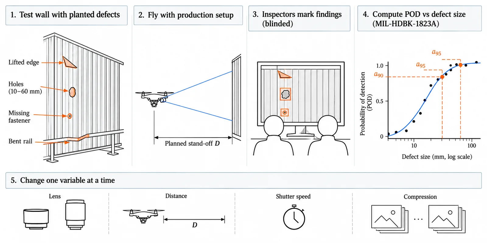
POD workflow: a test wall with planted defects, a drone flying the production setup, blinded inspectors marking findings, and a POD curve against defect size — The five steps of a POD trial.

The result tells you whether a better camera really moves the a90/95, the defect size found 90 % of the time with 95 % confidence, and it gives you a number to show an asset owner.

The size of the test matters. Finding 29 out of 29 planted defects of one size is enough to show a detection rate of at least 90 % at 95 % confidence. A trial planned to allow one miss needs 46 targets, and two misses need 61.

Light ruins more frames than resolution

The failures that never appear on a datasheet are about light.

Backlight is the first. Looking up at a chimney top, the camera exposed for the sky at 1/1600 s, f/5 and ISO 100, about EV 15.3, and the steel went almost black. Brightening it afterwards brings up noise and banding, not rust texture.

Shadow is the second. Gutters under the eaves, louvre interiors and the undersides of decks sit in deep shade next to sunlit roof, and a choked gutter you cannot see is a CAT-A you did not log.

Dust is the third. Plant dust turns everything pinkish grey. Auto white balance corrects for it differently from frame to frame, which destroys the colour that tells fresh rust from old paint.

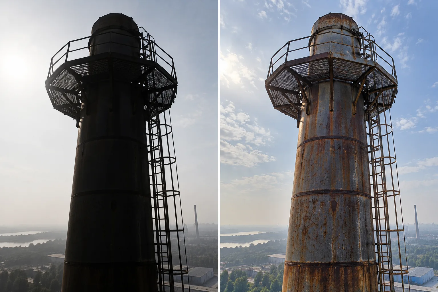
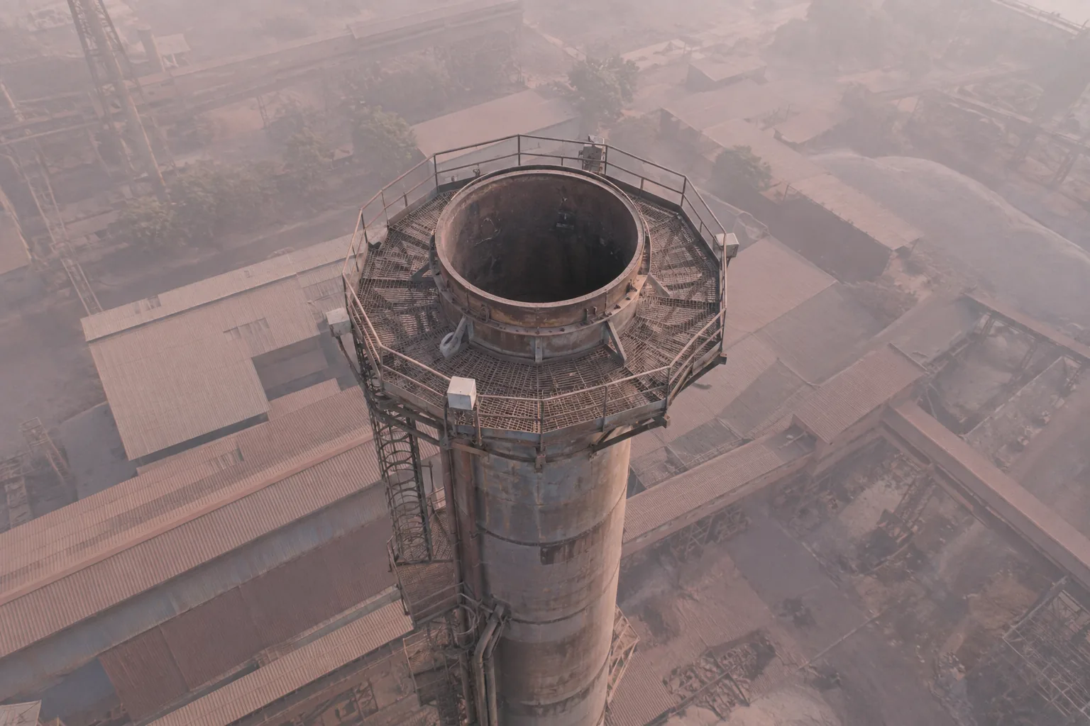
Two views of a steel stack: on the left exposed for the bright sky so the structure is a black silhouette, on the right exposed for the steel so rust is visible — Exposed for the sky (left) and for the steel (right).

A stack top seen through pinkish-grey plant dust haze — Plant dust shifts colour, and auto white balance shifts it differently every frame.

Three things help. The first is on-sensor HDR and larger pixels for backlit and shaded work. A 2.0 µm pixel collects about twice the light of a 1.4 µm one, and the IMX678 in e-con Systems’ e-CAM810 adds Clear HDR and DOL HDR modes.

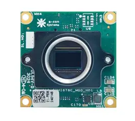
4K IMX678 low light and HDR
e-CAM810_CUMI678C_MOD
3840 × 2160 · 2 µm · rolling shutter · up to 72 fps at 4K
5.7 mm/pxat 17 m with a 6 mm lens, 21.8 m across
Product page

The second is white balance locked for the whole mission, set against a grey card at take-off, together with a tuned image pipeline. e-con Systems tunes colour for its cameras with its TintE ISP. The third is RAW 10 or 12 bit, or high-quality encoding. Dust surveys are a low-contrast problem, and heavy compression erases the texture that shows the ribs are still visible and the layer is thin.

Yearly inspections need a camera that does not drift

Most structures are inspected again on a schedule, often every year. The camera then becomes an instrument for measuring change, and an instrument must not drift.

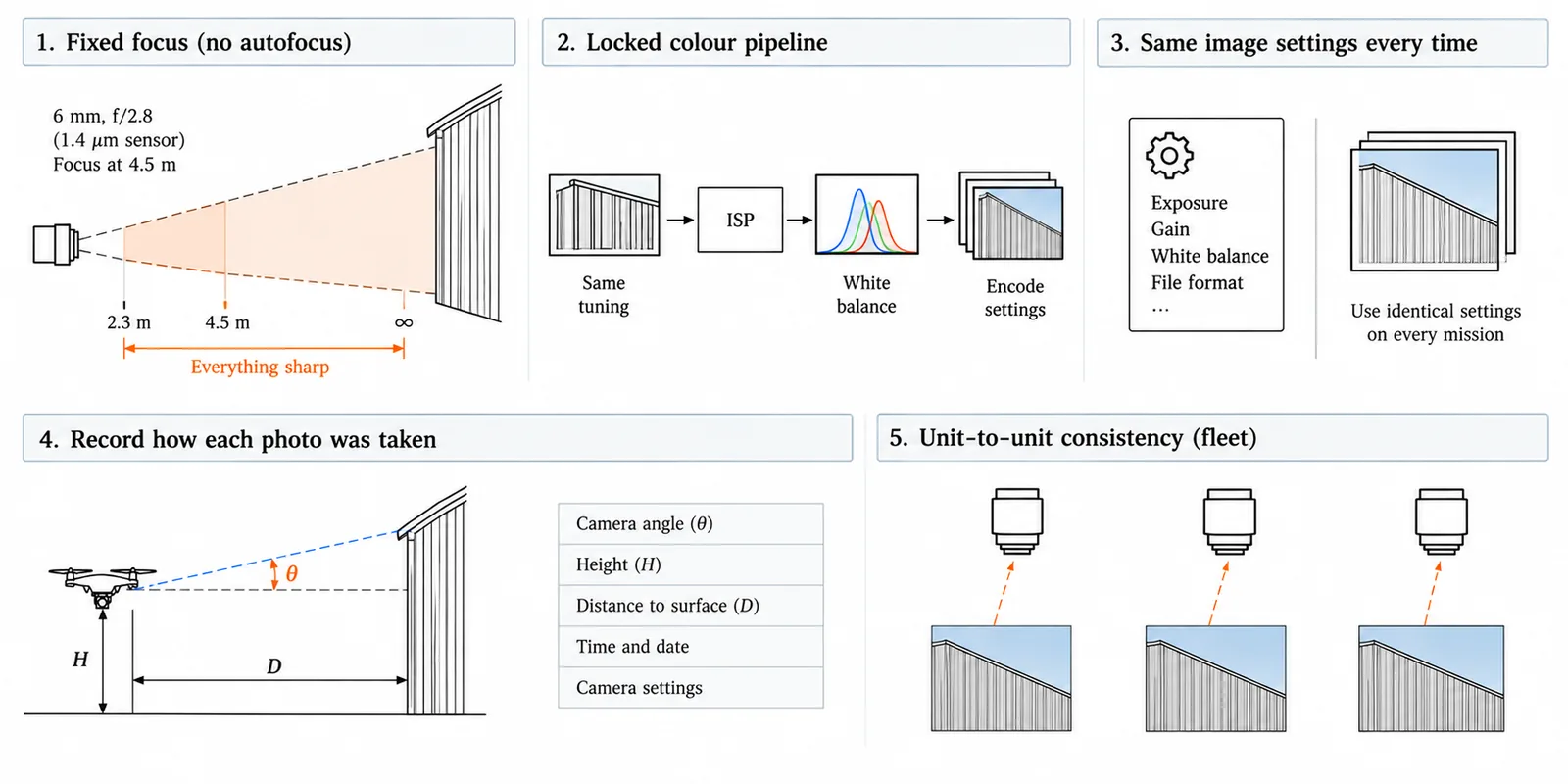
Fix the focus for the real inspection range instead of letting autofocus hunt across plain sheeting, so there is no focus difference between this year and next.
Keep the colour pipeline the same from mission to mission: same image tuning, same white balance method, same encoding settings.
Record how each photo was taken: camera angle, height, time and, if possible, the distance to the surface. Next year’s photo can then be matched to this year’s.
If you run a fleet, ask the vendor how colour and sharpness are held consistent across production units. That matters more than a headline spec.

Five practices for repeatable inspections: fixed focus, locked colour pipeline, same image settings, recorded capture geometry, unit-to-unit consistency — What keeps this year's frame comparable with next year's.

Close view of corroded corrugated cladding with streaks of rust — Corrosion is tracked as change over time, which only works if the camera does not drift.

Motion, vibration and the shutter

A moving drone blurs the image, and the blur depends on speed and exposure time. The arithmetic is short. At 4 mm per pixel, a drone drifting at 1 m/s during a 1/240 s exposure moves the image by about 4 mm, one pixel. Flying along a gallery at 2 m/s needs 1/1000 s to keep the blur to half a pixel. Gimbal jitter of 1° per second at 1/240 s adds about 0.3 pixel with a 6 mm lens, and it grows with focal length, so it gets worse when you fit a longer lens for more detail.

The card below does these sums for your own settings. It starts at 2 m/s and 1/1000 s, with the 6 mm lens at 17 m.

Motion blur

Motion

Speed m/s

Camera or subject. 0 if neither moves.

Shutter speed 1/x s

1000 means 1/1000 s.

Distance m

Straight line from the lens to the subject.

Camera

Focal length mm

Pixel size µm

From the sensor datasheet.

Combined blur

0.51 px

Blur from travel0.50 px2.00 mm during the exposure
Blur from shake0.07 px
Slowest shutter for 0.5 px1/1020 syours is 1/1000 s
Fastest speed for 0.5 px1.96 m/syours is 2.0 m/s

Speed against shutter for this lens and distance

Each line is a blur of 0.25, 0.5, 1 and 2 px for this lens and range. The shaded zone keeps blur under half a pixel. Lines drop away to the left because camera shake alone exceeds that blur at slow shutters. Your setup is the dot.

Show the numbers

Ground sample distance3.97 mm/px

Travel during exposure2.00 mm

Travel and shake blur are independent and add in quadrature. Rolling-shutter skew and the noise cost of short exposures are not modelled.

Equations

Pixel size on the surface: $GSD = \frac{(R - f) \cdot p}{f}$ GSD = (R − f) · p ÷ fR is the distance from the lens and p the pixel pitch, in the same unit as f.
Blur from travel: $L_{travel} = \frac{v \cdot t}{GSD}$ L_travel = v · t ÷ GSDv is the speed, t the exposure time and GSD the pixel size on the surface, in matching length units. L is in pixels.
Blur from shake: $L_{shake} = \frac{f \cdot ω \cdot t}{p}$ L_shake = f · ω · t ÷ pω is the rotation rate in radians per second and p the pixel pitch, in the same unit as f. L is in pixels.
Combined blur: $blur = \sqrt{{L_{travel}}^{2} + {L_{shake}}^{2}}$ blur = sqrt(L_travel² + L_shake²)The two blurs are independent, so they add in quadrature. Blur is in pixels.
Slowest shutter for 0.5 px: $t = \frac{0.5}{\sqrt{{(\frac{v}{GSD})}^{2} + {(\frac{f \cdot ω}{p})}^{2}}}$ t = 0.5 ÷ sqrt((v ÷ GSD)² + (f · ω ÷ p)²)The shutter speed shown is 1 ÷ t.
Fastest speed for 0.5 px: $v = \frac{GSD \cdot \sqrt{{0.5}^{2} - {L_{shake}}^{2}}}{t}$ v = GSD · sqrt(0.5² − L_shake²) ÷ tApplies while shake alone is under 0.5 px; above that no speed reaches 0.5 px.

Sharpness also depends on the lens and the aperture. Diffraction sets a hard limit: with 1.4 µm pixels at f/5.6, contrast falls to zero at 0.455 cycles per pixel, just below the 0.5 the sensor can sample, so the finest tenth of the band is already empty before any lens flaw. Focus errors cost contrast in the same way.

The next card adds up every loss between the wall and the sensor. It starts at f/5.6 with 1.4 µm pixels, a 6 mm lens and a 17 m stand-off.

Sharpness budget

Camera and lens

Pixel size µm

From the sensor datasheet.

Focal length mm

Aperture f/

f/5.6 means 5.6.

Distance and focus

Distance m

Focused at

Motion

Speed m/s

Camera or subject. 0 if neither moves.

Shutter speed 1/x s

1000 means 1/1000 s.

Effective pixel size on the surface

7.70 mm

Nominal pixel size3.97 mm
Contrast at Nyquist0 %pixel aperture alone: 64 %
Usable limit (20 % contrast)0.26 cy/pxNyquist is 0.5 cy/px
Diffraction limitf/2.1yours is f/5.6

Contrast against spatial frequency

Contrast kept at each spatial frequency. Dark line: the whole chain, every component multiplied. Dashed: the pixel aperture alone. Detail finer than the usable limit, where contrast falls to 20 %, is lost in noise.

Contrast at Nyquist, by cause

Diffraction0 %
Pixel aperture64 %
Lens aberrations29 %
Defocus100 %
Movement90 %
Camera shake100 %
Whole chain0 %

Show the numbers

MTF500.15 cy/px

Airy disc7.52 µm5.4 px

Hyperfocal distance4.6 m

Depth of field3.62–∞ msubject inside

Defocus at subject0.00 pxblur circle

Components multiply along the axis of motion, the worst case. Defocus is geometric (a uniform disc), diffraction is an ideal circular aperture, and lens aberrations are one Gaussian that you set from the lens datasheet or a test chart. ISP sharpening, denoising, Bayer demosaicing and the optical low-pass filter are not modelled.

Equations

Whole system: $MTF (ν) = {MTF}_{dif} \cdot {MTF}_{pix} \cdot {MTF}_{lens} \cdot$
${MTF}_{defocus} \cdot {MTF}_{move} \cdot {MTF}_{shake}$ MTF(ν) = MTF_dif · MTF_pix · MTF_lens · MTF_defocus · MTF_move · MTF_shakeν is the spatial frequency in cycles per pixel. Nyquist is 0.5. The parts multiply.
Diffraction: ${MTF}_{dif} = \frac{2}{π} (\arccos x - x \cdot \sqrt{1 - x^{2}}), x = \frac{ν \cdot λ \cdot N}{p}$ MTF_dif = (2 ÷ π) · (arccos x − x · sqrt(1 − x²)), x = ν · λ · N ÷ pN is the f-number; λ and p share one unit. The value is 0 once x reaches 1.
Pixel aperture: ${MTF}_{pix} = | \frac{\sin (π ν)}{π ν} |$ MTF_pix = |sin(πν) ÷ (πν)|
Movement: ${MTF}_{move} = | \frac{\sin (π ν L)}{π ν L} |$ MTF_move = |sin(πνL) ÷ (πνL)|, with L = v · t ÷ GSDL is the blur length in pixels, v · t ÷ GSD as in the motion tool.
Camera shake: ${MTF}_{shake} = | \frac{\sin (π ν L)}{π ν L} |$ MTF_shake = |sin(πνL) ÷ (πνL)|, with L = f · ω · t ÷ pL is the blur length in pixels, f · ω · t ÷ p as in the motion tool.
Defocus: ${MTF}_{defocus} = | \frac{2 \cdot J₁ (x)}{x} |, x = π ν c$ MTF_defocus = |2 · J1(x) ÷ x|, x = πνcc is the blur circle in pixels and J1 the first-order Bessel function.
Blur circle: $c = \frac{f^{2} \cdot | d - s |}{N \cdot d \cdot (s - f) \cdot p}$ c = f² · |d − s| ÷ (N · d · (s − f) · p)d is the distance to the object and s the distance focused at, in the same unit as f; p is the pixel pitch in that unit.
Lens blur: ${MTF}_{lens} = \exp (- 2 π^{2} σ^{2} ν^{2})$ MTF_lens = exp(−2π²σ²ν²)σ is the lens blur as a Gaussian, in pixels.
Hyperfocal distance: $H = \frac{f^{2}}{N \cdot p} + f$ H = f² ÷ (N · p) + fOne pixel is taken as the acceptable blur.
Near and far focus limits: $near = \frac{s (H - f)}{H + s - 2 f}, far = \frac{s (H - f)}{H - s}$ near = s · (H − f) ÷ (H + s − 2f), far = s · (H − f) ÷ (H − s)Far is unlimited when s is at or beyond H.
Airy disc: $d = 2.44 \cdot λ \cdot N$ d = 2.44 · λ · NThe disc spans 2 pixels when N = 2p ÷ (2.44 λ).
Effective pixel size: ${GSD}_{eff} = GSD \cdot \max (1, \frac{1}{2 ν_{limit}})$ GSD_eff = GSD · max(1, 1 ÷ (2 · ν_limit))ν_limit is where the whole-system MTF falls to the chosen contrast.

The right shutter type depends on the camera’s job.

For inspection photos, a high-resolution rolling-shutter sensor works well while the drone hovers.
For navigation and obstacle cameras, use a global shutter. A rolling shutter reads the image line by line, so fast movement bends straight edges, and that confuses navigation software (see rolling shutter). Stereo pairs also have to capture at the same moment. Two unsynchronised cameras at 60 fps can be up to one frame apart, 16.7 ms, and that is enough to create false depth when the drone is moving.

Two e-con Systems modules fit this job: the e-CAM217 (AR0234, 1920 × 1200 at 60 fps) for plain navigation and the e-CAM521 (IMX568, 5 MP) when stereo or navigation needs more resolution.

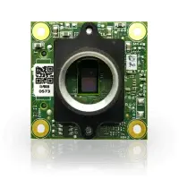
AR0234 global shutter
e-CAM217_CUMI0234_MOD
1920 × 1200 · 3 µm · global shutter · 60 fps at 1920 × 1200
8.5 mm/pxat 17 m with a 6 mm lens, 16.3 m across
Product page
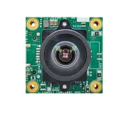
5 MP IMX568 global shutter
e-CAM521_CUMI568C_MOD
2472 × 2064 · 2.74 µm · global shutter · 79 fps at 5 MP
7.8 mm/pxat 17 m with a 6 mm lens, 19.2 m across
Product page

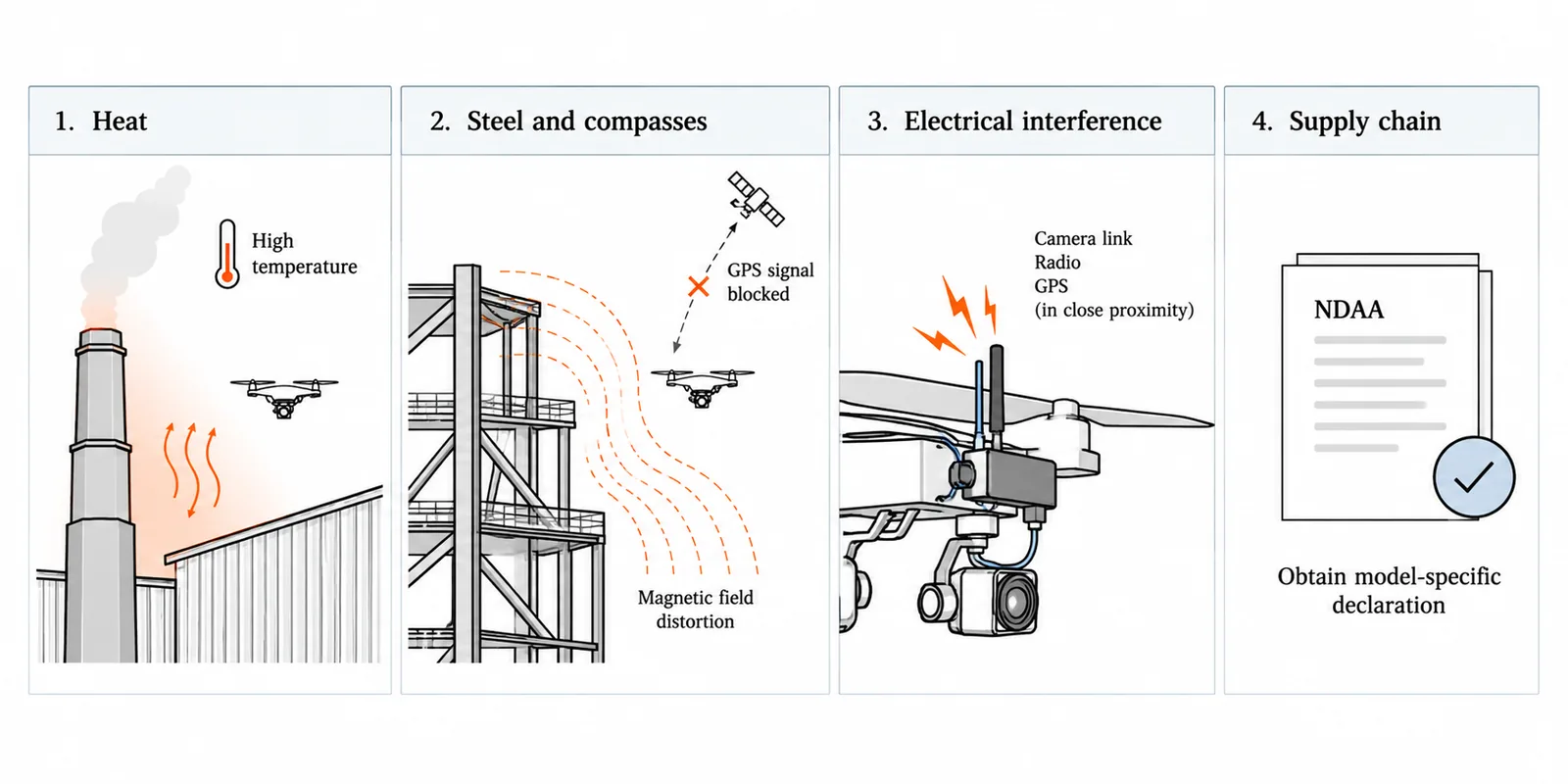
Heat, steel and interference

Heat: cast houses, stacks and hot-gas ducts raise the local air temperature well above ambient. Check the exact rating against your flight conditions and give the camera airflow in the payload design.
Steel and compasses: large steel structures distort the magnetic field a drone’s compass relies on, and tall structures can block satellite signals. That is exactly where you inspect, and it is why navigation from cameras is worth having.
Electrical interference: fast camera links sit next to radios and GPS. Ask for EMC test documents for the exact camera model, and test the complete payload yourself.
Supply chain: if your programme has NDAA requirements, ask for a declaration for the specific model, not a general claim.

Four payload risks: heat near stacks, steel structures disturbing compass and GPS, electrical interference from camera links, and supply-chain declarations — The payload risks that show up at inspection range.

Plan the data before the drone

A serious inspection drone often carries several cameras, each with its own job. This example rig uses e-con Systems cameras, and the plate shows the raw data it produces.

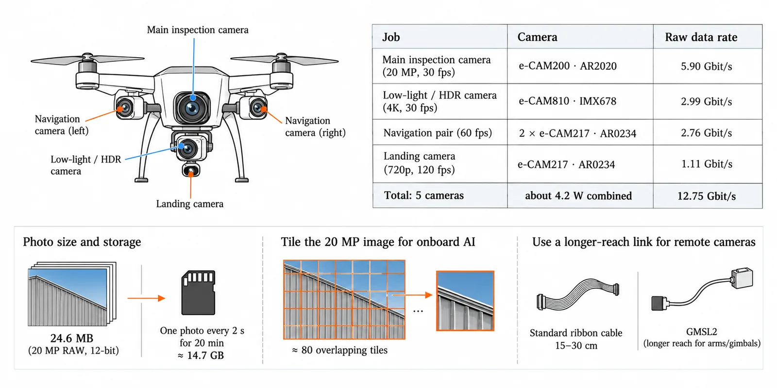
A five-camera inspection drone: 20 MP inspection camera at 5.90 Gbit/s, 4K HDR camera at 2.99 Gbit/s, a navigation pair at 2.76 Gbit/s and a landing camera at 1.11 Gbit/s, 12.75 Gbit/s in total — Five cameras, 12.75 Gbit/s of raw data.

Three numbers are worth bringing to the first design meeting.

12.75 Gbit/s decides how you connect the cameras and which computer you need on board.
24.6 MB is one 20 MP RAW photo at 10 bit. One photo every 2 seconds on a 20-minute flight comes to about 14.7 GB, so decide early what you keep.
80 tiles is what it takes to run defect detection on the drone without shrinking the photo. Squeezed to a 640-pixel-wide model input, 4 mm per pixel becomes 32 mm per pixel and small defects vanish. Cutting the photo into 640-pixel tiles with 20 % overlap takes about 80 tiles and keeps the detail.

Change the cameras, the flight or the model input size to see how the numbers move. The card starts with the five-camera rig above, with the e-CAM200 as the inspection camera.

Data path

Cameras
Camera	Gbit/s	Fits on
Camera 119.7 MP	5.90	CSI-2 ×4
Camera 28.3 MP	2.99	USB 3
Camera 32.3 MP	2.76	USB 3 ×2
Camera 40.9 MP	1.11	USB 3

Bus and storage

Pixels on the bus

Packed carries 10 or 12 bits per pixel as captured. Many drivers pad to 16 bits in memory.

Recording time min

Still every s

Model input size px

Total data rate

12.8 Gbit/s

Largest stream: Camera 1CSI-2 ×45.90 Gbit/s per camera; cheapest link that carries it
Storage for 20 min1913 GBall streams, 1.59 GB/s
Camera 1 stills for 20 min14.7 GB600 frames of 24.6 MB
Tiles per Camera 1 frame80640 px tiles, 20 % overlap

Data rate by camera

Tiling of one Camera 1 frame

80 tiles of 640 px with 20 % overlap cover one frame without shrinking it. Shrinking the frame to 640 px instead makes pixels 8.0× coarser.

Show the numbers

One RAW frame, Camera 124.6 MB

All streams1.59 GB/s

Uncompressed. Link capacity is the nominal line rate with 20 % held back for protocol overhead and headroom; sustained payload depends on your SoC and drivers, so measure on the hardware. Compression, binning and crops are not modelled.

Equations

Data rate of one camera: $Gbit/s = \frac{W \times H \times b \times fps}{10^{9}}$ Gbit/s = W × H × b × fps ÷ 10^9W and H are pixels, b the bits per pixel on the bus and fps the frame rate. The total is the sum over the cameras.
Storage: $GB = \frac{Gbit/s \times 60 \times T}{8}$ GB = Gbit/s × 60 × T ÷ 8Gbit/s is the total over all cameras and T the recording time in minutes.
One still frame: $MB = \frac{W \times H \times b}{8 \times 10^{6}}$ MB = W × H × b ÷ (8 × 10^6)Decimal megabytes. Stills over time: frames = 60 × T ÷ interval.
Tiles across the frame: $tiles across = ⌈ \frac{W - t}{0.8 \cdot t} ⌉ + 1$ tiles across = ceiling((W − t) ÷ (0.8 · t)) + 1t is the tile size in pixels and 0.8 leaves a 20 % overlap. Tiles down use H. Tiles per frame = across × down.
Usable link capacity: $usable = 0.8 \times line rate$ usable = 0.8 × line rateA camera fits a link when its data rate is at or below this.

Cable length matters too. Standard camera ribbon cables are only 15 to 30 cm long. For cameras on arms or gimbals, use GMSL2, a camera link that reaches further.

The camera was not the only bottleneck

On industrial sites, inspection days are lost to permits, weather, batteries and interference far more often than to the camera. A camera cannot shorten a permit queue. What it can do is raise the chance that one 20-minute flight produces usable evidence, because a re-flight costs another permit and another weather window.

Specifying the camera

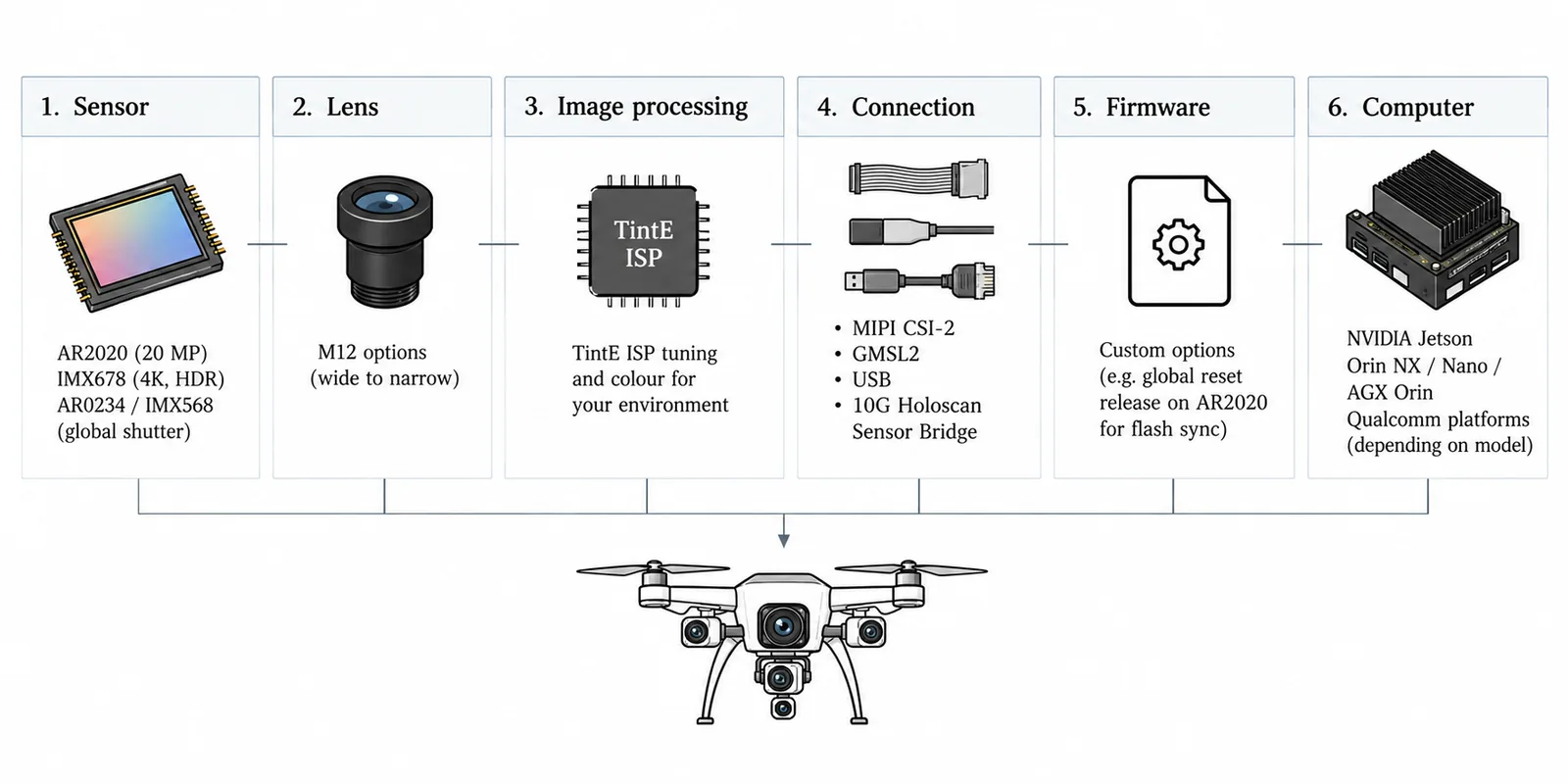
Image quality comes from the sensor, lens, image processing, cable and firmware working together, and that is how e-con Systems designs its cameras. Around the sensors above it offers M12 lens options from wide coverage to narrow detail, colour tuning for your site, MIPI CSI-2, GMSL2, USB and 10G Holoscan Sensor Bridge connections depending on the model, custom firmware (for example a global reset release on the AR2020 for flash-synchronised photos), and support for NVIDIA Jetson Orin NX, Nano and AGX Orin and Qualcomm platforms. Availability depends on the model, so check the product pages.

Six parts of a camera specification: sensor, lens, image processing, connection, firmware and computer — Image quality comes from six parts working together.

Questions to ask a drone camera vendor

What GSD do I get at my real stand-off with the lens you propose?
Which lenses can you supply for 10 m, 17 m and 30 m stand-off, and what is their MTF at the sensor’s Nyquist frequency?
Which HDR modes does the camera expose on my computing platform, and at what frame rates?
Can I lock white balance, exposure and image settings for a whole mission, and can I export RAW?
Which sensors are global shutter, and can they be synchronised in hardware?
What is the readout time in the mode I will use, and what does it mean for motion distortion?
What cable lengths do you support, and is GMSL2 available?
What is the operating temperature range of the exact model I am buying?
What are the power draw and weight with the lens fitted?
Can you provide EMC, environmental and NDAA documentation for the exact model?
How do you keep colour, focus and sharpness consistent across cameras in a fleet?
Will you help me measure POD on a seeded test wall, at my real stand-off, speed and lighting?

Making training data when real defects are rare

If you are building AI to find defects, you will hit a familiar problem. Real defect photos are rare, they belong to the asset owner, and they are unevenly spread. There are thousands of photos of sound walls and very few of torn sheets.

We built a casebook of 16 inspection scenarios, from loose cladding to backlit chimney tops. Each one fixes the camera angle, stand-off, defect size, lighting and the visual limits that make an image behave like a real inspection frame. Drawing a torn sheet is not enough. The distance, perspective, light, material and surroundings have to be controlled as well. A training image for a torn conveyor-gallery sheet, for example, might be specified like this:

17 m stand-off · 35° camera tilt · ~400 mm tear · low-angle light · corrugated steel · handrail and walkway in frame

Want the full defect casebook? The 16 scenarios, with their prompts and constraints.

Request the casebook

Artifacts

Defect casebook: 16 inspection scenarios (on request)documentPixel budget: check a frame from your own dronetool

Cite this

@article{beyondpixels_steel_plant_drone_frames,
  title   = {What Thousands of Steel-Plant Drone Frames Reveal About the Camera and AI You Actually Need},
  author  = {Sumit Kumar},
  journal = {Beyond Pixels},
  year    = {2026},
  url     = {https://beyondpixels.dev/blog/steel-plant-drone-frames/}
}

Start from the defect

20 MP AR2020

The emergencies are on the walls

What 4 mm per pixel can and cannot show

56 mm

Common details at this pixel size

Measure the probability of detection

Light ruins more frames than resolution

4K IMX678 low light and HDR

Yearly inspections need a camera that does not drift

Motion, vibration and the shutter

0.51 px

Speed against shutter for this lens and distance

7.70 mm

Contrast against spatial frequency

Contrast at Nyquist, by cause

AR0234 global shutter

5 MP IMX568 global shutter

Heat, steel and interference

Plan the data before the drone

12.8 Gbit/s

Data rate by camera

Tiling of one Camera 1 frame

The camera was not the only bottleneck

Specifying the camera

Questions to ask a drone camera vendor

Making training data when real defects are rare

Artifacts

Cite this